Solving a Statically Indeterminate Problem Using Compatibility

A Step-by-Step Mechanics of Materials Example (Hibbeler 9th Edition)

In this post, we solve a statically indeterminate mechanics of materials problem using equilibrium and compatibility equations. The example, taken from Hibbeler, Mechanics of Materials (9th Edition), is presented step by step with an emphasis on clear reasoning and physical interpretation.

Introduction

Statically indeterminate problems are a common source of difficulty for students in Mechanics of Materials because they cannot be solved using equilibrium equations alone. In such problems, the number of unknown forces exceeds the number of available equilibrium equations, requiring an additional physical principle to reach a solution.

We begin by applying the equations of static equilibrium and quickly discover that they are insufficient on their own, which naturally leads to the concept of compatibility of deformation.

The solution is presented step by step, starting with the free-body diagram and equilibrium equations, and progressing toward the compatibility condition and final results. Throughout the discussion, emphasis is placed on both the mathematics and the physical meaning of each step, helping you build a deeper understanding of statically indeterminate systems and learn to apply compatibility conditions systematically.

The following video walks through the complete solution step by step, explaining both the mathematical procedure and the underlying physical reasoning.

The remainder of this post explains the same solution in written form, so you can follow each step of the reasoning at your own pace and refer back to key ideas as needed.

Problem Description

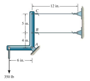
This problem examines a rigid L-shaped link supported by a pin at point A and connected to two horizontal steel wires at points B and C (Figure 1). The wires are attached to a fixed support on the right and can carry only tensile forces. A vertical load of 350 lb is applied downward at the end of the horizontal segment of the rigid link.

Both steel wires have identical material and geometric properties: each has an unstretched length of 12 in, a cross-sectional area of 0.0125 in², and is made of A-36 structural steel.

The objective of the problem is to determine the forces developed in the two steel wires when the 350-lb load is applied. Equilibrium equations alone are insufficient, and an additional condition based on deformation compatibility is required.

This type of structural configuration is common in mechanical and civil engineering applications, including crane support systems, aircraft control linkages, and tension-rod bracing in buildings. Understanding how to analyze such systems is essential for designing safe and efficient structures.

System Geometry and Physical Setup

The configuration of the system is shown in Figure 1. The rigid link is pinned at point A, which prevents translation of the link but allows it to rotate freely. Two horizontal steel wires are attached to the link at points B and C and are anchored to a rigid support on the right.

The geometry of the link is defined by the vertical distances between these points. Point B is located 4 in above the pin at A, while point C is located an additional 5 in above point B, placing point C a total of 9 in above point A. These distances are important because they determine how much each attachment point moves when the link rotates.

A vertical load of 350 lb is applied at the end of the horizontal segment of the link. The horizontal distance from the line of action of this load to the pin at A is 6 in, which defines the moment arm of the applied load about the pin.

The rigid link is assumed to remain undeformed under loading; that is, it neither stretches nor bends. Instead, when the external load is applied, the link undergoes a small rotation about point A.

Free Body Diagram (FBD)

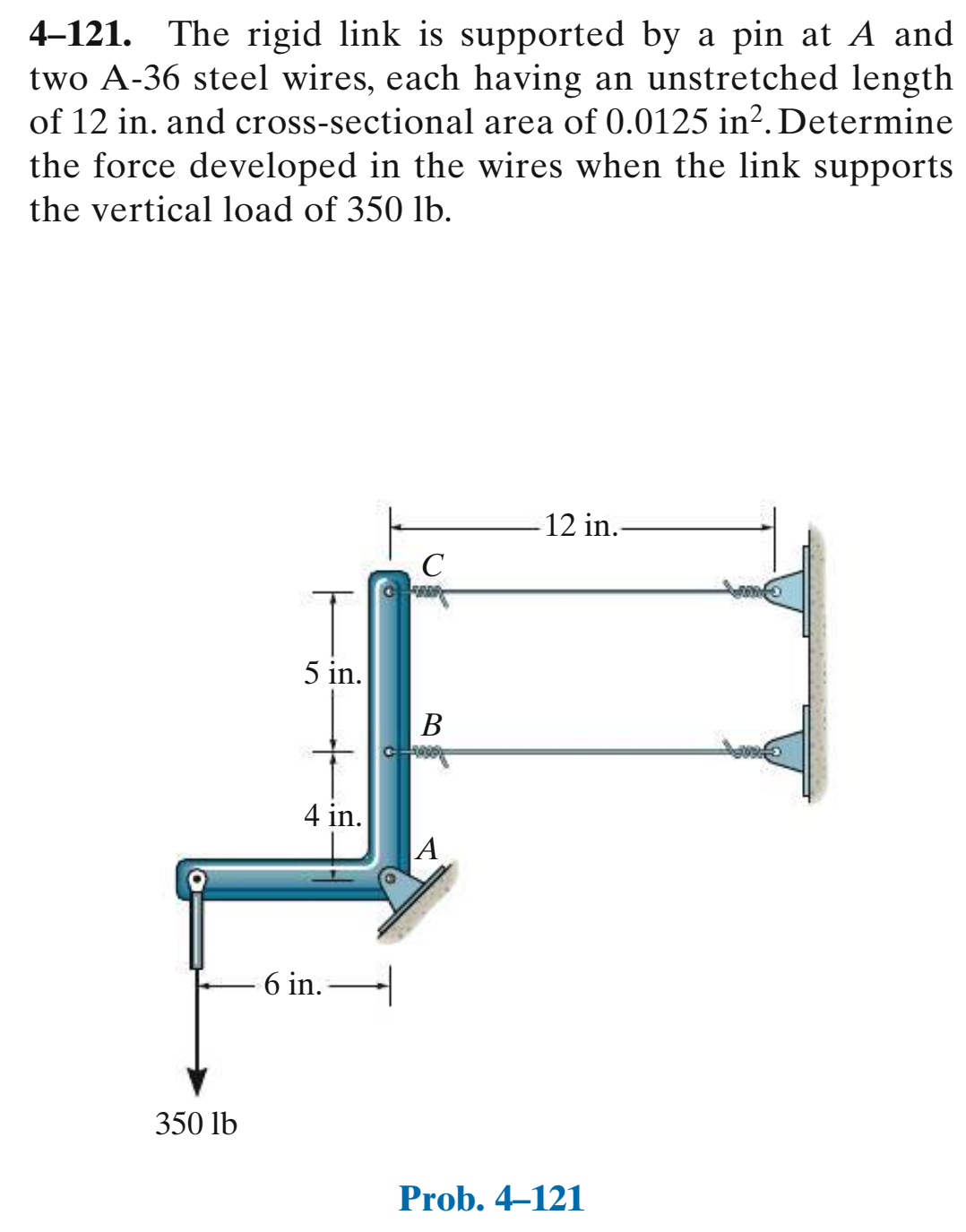
To analyze the forces acting on the structure, we begin by isolating the rigid link and constructing its free body diagram, shown in Figure 2.

In the free body diagram, the rigid L-shaped link is isolated from its supports, and all external forces acting on it are explicitly shown. The pin at point A provides two reaction components: a horizontal reaction $A_x$​ and a vertical reaction $A_y$​. Because the pin allows rotation but prevents translation, no moment reaction exists at point A.

The two horizontal steel wires exert tensile forces $T_B$ and $T_C$ on the link at points B and C, acting horizontally toward the fixed support. Since the wires can carry only axial tension, these forces are purely horizontal.

An external vertical load of 350 lb is applied downward at the end of the horizontal segment of the link, with a moment arm of 6 in about point A.

At this stage, the free body diagram makes it clear that the unknown forces acting on the link include the wire tensions $T_B$​ and $T_C$​, as well as the pin reactions $A_x$​ and $A_y$​. However, since the objective is to determine the forces in the wires, the equilibrium equations will be written in a way that eliminates the pin reactions from the analysis.

Equilibrium Equations

With the free body diagram established (Figure 2), we now apply the equations of static equilibrium to the rigid link.

Although the pin at point $A$ provides two reaction components $A_x$​ and $A_y$​, our primary objective is to determine the tensions in the two steel wires, $T_B$​ and $T_C$​. For this reason, we select an equilibrium equation that eliminates the unknown pin reactions from the analysis.

The most effective equilibrium equation for this system is the moment equilibrium about point A. Taking moments about the pin has a key advantage: the reaction forces $A_x$ and $A_y$ produce no moment about point A and therefore do not appear in the equation. (We’ll use the convention that counterclockwise moments are positive.)

From the free body diagram:

• The tension force $T_B$​ acts horizontally at point $B$, located 4 in above point A. Its moment about $A$ is clockwise.
• The tension force $T_C$​ acts horizontally at point $C$, located 9 in above point A. Its moment about $A$ is also clockwise.
• The applied load of 350 lb acts downward at a horizontal distance of 6 in from point $A$, producing a counterclockwise moment.

Writing the moment equilibrium equation about point $A$:

∑𝑀_𝐴=0

-𝑇_𝐵(4)−𝑇_𝐶(9)+350(6)=0

Rearranging,

4T_B + 9T_C = 2100\ \ \ \ \ (lb.in)

At this stage, the equilibrium analysis yields one equation containing two unknowns, $T_B$​ and $T_C$​, which confirms that the system is statically indeterminate and cannot be solved using equilibrium alone; an additional equation derived from deformation compatibility is required to complete the solution.

In the next section, we develop this required compatibility relationship by examining the small rotation of the rigid link and the resulting elongations of the two steel wires.

With one equation and two unknowns established, we now turn to the physical deformation of the system to develop our second equation.

Deformation and Compatibility Concept

Because the equilibrium equation alone is insufficient to determine the forces in the two wires, an additional relationship based on deformation compatibility must be introduced.

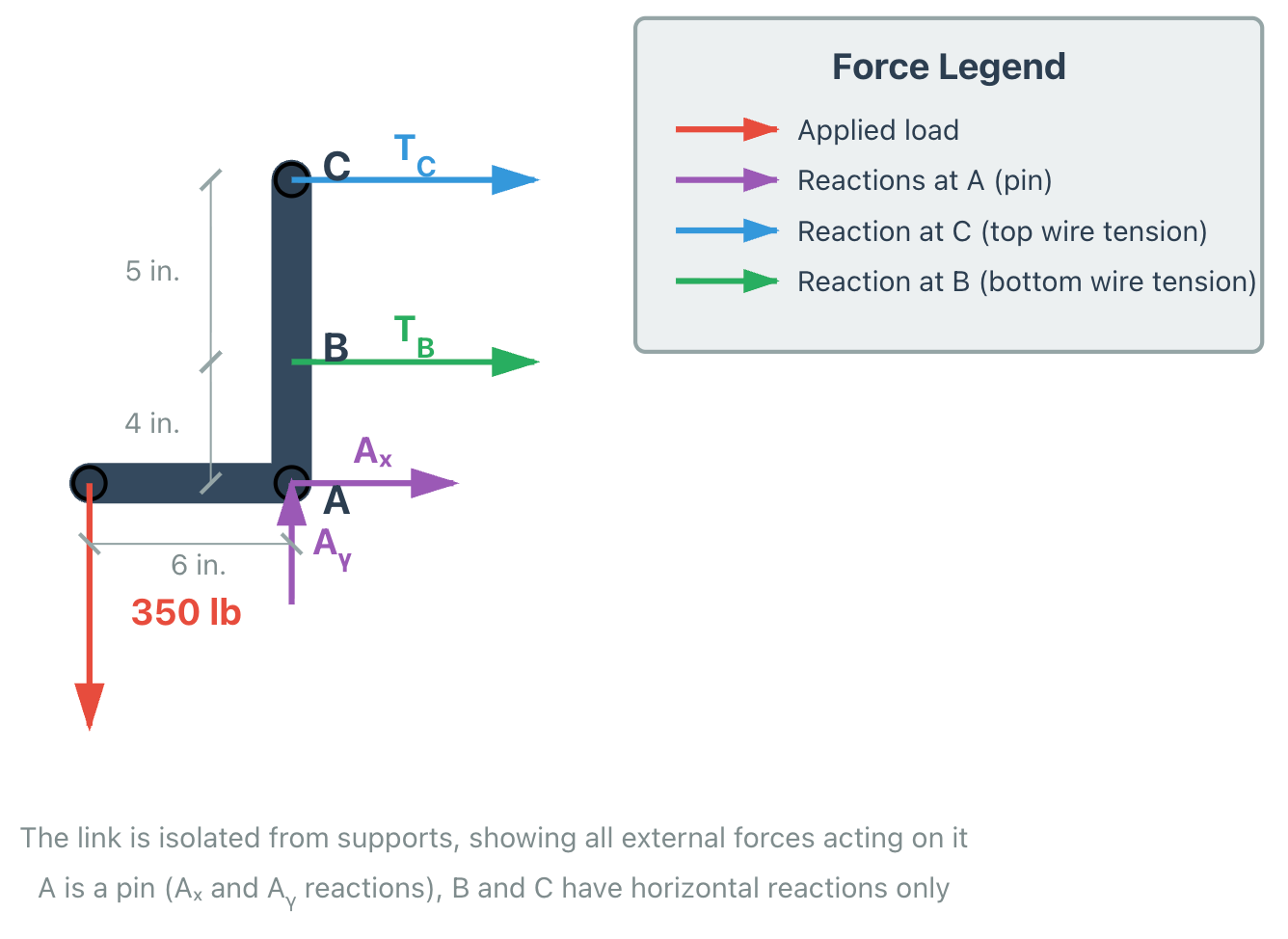
The rigid L-shaped link is assumed to remain undeformed under loading; that is, it does not stretch or bend. Instead, when the 350-lb vertical load is applied, the link undergoes a small rotation about the pin at point A (Figure 3). This rotation produces horizontal displacements at points B and C, which in turn cause axial deformations in the two steel wires. These geometric displacement relationships form the foundation of the compatibility condition.

Since the rotation of the link is small, the resulting displacements can be related using simple geometry. Let the rigid link rotate through a small angle $\theta$ about point A. The horizontal displacement at each wire attachment point is then proportional to its vertical distance from the pin:

• The displacement at point B is:

\delta_B = AB \cdot \theta

• The displacement at point C is:

\delta_C = AC \cdot \theta

Because both displacements arise from the same rigid-body rotation, the angle $\theta$ is common to both expressions. Taking the ratio of the two displacements eliminates the rotation angle and yields a direct geometric relationship between them:

\frac{\delta_C}{\delta_B} = \frac{AC}{AB}

Using the known geometry of the link,

\frac{\delta_C}{\delta_B} = \frac{9\,^{in}}{4\,^{in}}

which can be written as the compatibility equation:

4\,\delta_C = 9\,\delta_B

This compatibility condition reflects the physical requirement that the deformations of the two wires must be consistent with the rigid rotation of the link. In the following section, this geometric relationship will be combined with the axial deformation formulas for the wires to obtain the second equation needed to solve the problem.

Wire Deformation Using Hooke’s Law

To convert the geometric compatibility condition into a force relationship, we relate the axial deformation of each steel wire to the force it carries using Hooke’s law.

For a prismatic bar subjected to an axial force, the elongation is given by:

\delta = \frac{PL}{EA}

where:

• $P$ is the axial force in the member,
• $L$ is the original length,
• $E$ is the modulus of elasticity, and
• $A$ is the cross-sectional area.

Applying this expression to the two steel wires:

• Wire at point B:

\delta_B = \frac{T_B L}{EA}

• Wire at point C:

\delta_C = \frac{T_C L}{EA}

Since both wires have identical properties (same E, L, and A as specified earlier), these quantities will cancel out when we combine compatibility with Hooke’s law.

From the compatibility analysis, the horizontal displacements satisfy:

4\,\delta_C = 9\,\delta_B

Substituting the expressions from Hooke’s law:

4\left(\frac{T_C L}{EA}\right) = 9\left(\frac{T_B L}{EA}\right)

Since $L$, $E$, and $A$ are the same for both wires, they cancel, yielding a force-based compatibility equation:

4T_C = 9T_B

At this stage, the problem is reduced to two equations:

• From equilibrium:

4T_B + 9T_C = 2100 \,\text{lb.in}

• From compatibility:

4T_C = 9T_B

These two equations can now be solved simultaneously to determine the forces in the two wires.

Solving the System of Equations

From the preceding sections, we have obtained two independent equations governing the unknown wire tensions $T_B$​ and $T_C$​:

• Equilibrium equation (moment equilibrium about point $A$)
• Compatibility equation (geometric compatibility of wire deformations)

Together, these form the following system of equations:

\left\{
\begin{aligned}
4T_B + 9T_C &= 2100 && \text{(equilibrium)} \\
4T_C       &= 9T_B  && \text{(compatibility)}
\end{aligned}
\right.

This system contains two equations and two unknowns and can now be solved using standard algebraic techniques.

From the compatibility equation,

T_C = (\frac{9}{4})T_B

Substituting this expression into the equilibrium equation gives:

4T_B + 9\left[(\frac{9}{4})T_B\right] = 2100

Simplifying,

4T_B + (\frac{81}{4})T_B = 2100

Factoring out $T_B$,

\left(4 + \frac{81}{4}\right)T_B = 2100

(\frac{97}{4})T_B = 2100

Solving for $T_B$​,

T_B = \frac{2100 \times 4}{97} \approx 86.6 \ \text{lb}

Using the compatibility relation,

T_C = (\frac{9}{4})T_B = \frac{9}{4}(86.6) \approx 195 \ \text{lb}

Final Results

By combining the equations of static equilibrium with the deformation compatibility condition, the forces developed in the two steel wires have been fully determined.

The resulting wire tensions are:

\boxed{ \begin{aligned} T_B &\approx 86.6 \ \text{lb} \\ T_C &\approx 195 \ \text{lb} \end{aligned} }

Verification:

We can verify these results satisfy both governing equations:

Equilibrium check:

4(86.6) + 9(195) = 346.4 + 1755 = 2101.4 ≈ 2100 ✓

Compatibility check:

4(195) = 780\\
9(86.6) = 779.4 ≈ 780 ✓

The small discrepancies are due to rounding in the intermediate steps.

Although the two wires are identical in material, cross-sectional area, and original length, they do not carry equal forces. The difference in tension arises entirely from the geometry of the rigid link and the resulting kinematic relationship between the wire displacements.

Because the rigid link rotates about point $A$, the horizontal displacement at point $C$ is greater than that at point $B$. This larger displacement causes a greater axial deformation in the upper wire, which in turn produces a higher tensile force in wire $C$.

These results highlight a key principle in statically indeterminate systems:

Force distribution is governed not only by equilibrium, but also by deformation compatibility.

Common Mistakes to Avoid

• Over-relying on equilibrium equations
  In statically indeterminate systems, equilibrium provides fewer equations than unknowns. You must include deformation compatibility. Taking moments about point A eliminates pin reactions and is typically the most efficient equilibrium equation.
• Assuming equal wire forces because the wires are identical
  Even though both wires have the same length, cross-sectional area, and material, they experience different elongations due to their different distances from the pin. Identical material and geometrical properties do not imply equal forces.
• Mixing compatibility and constitutive equations
  Compatibility equations come from geometry and kinematics (how the structure moves), while Hooke’s law relates force to deformation. Write these separately, then combine them systematically.
• Jumping to algebra without physical interpretation
  Solving equations mechanically without understanding what the deformations and forces represent physically often leads to setup errors. Always pause to interpret what each equation means in terms of the structure’s behaviour.

Closing Remarks

This step-by-step strategy, combining equilibrium with compatibility, is a powerful framework that extends to more complex problems, including indeterminate beams, frames, and truss systems. Real-world applications include crane design, aircraft structures, suspension bridges, and building bracing systems.

As you practice similar problems, focus not only on obtaining numerical answers but also on understanding the physical behaviour. Ask yourself: Why does this wire carry more force? How would the solution change if the geometry were different? This deeper reasoning is what separates mechanical problem-solving from true engineering understanding.

Next Steps: Try solving a similar problem independently, sketching the deformed shape before writing equations, and checking that your final forces satisfy both equilibrium and compatibility.